Still working our way through this tutorial based on C++ and MINUIT:
http://www.desy.de/~rosem/flc_statistics/data/04_parameters_estimation-C.pdf
Now, we tackle the L3 LEP data.
L3 was an experiment at the Large Electron Positron collider, at CERN, near Geneva.
Until 2000, it recorded the decay products of e+e- collisions at center of mass energies up to 208 GeV.
An example is the muon pair production:
Both muons are mainly detected and reconstructed from the tracking system. From the measurements, the curvature, charge and momentum are determined.
The file L3.dat contains recorded muon pair events.
Every line is an event, a recorded collision of a \(e^+e^-\) pair producing a \(\mu^+\mu^-\) pair.
The first three columns contain the momentum components \(p_x\), \(p_y\) and \(p_z\) of the \(\mu^+\).
The other three columns contain the momentum components for the \(mu^-\).
Units are in \(GeV/c\).
Forward-Backward Asymmetry
An important parameter that constrains the Standard Model (the theoretical framework that models our current understanding of Physics) is the forward-backward asymmetry A:
where:
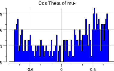
\(N_F\)are the events in which the\(\mu^-\)flies forwards (\(\cos \theta_{\mu^-} > 0\));\(N_B\)are the events in which the\(\mu^-\)flies backwards.
Given the L3.dat dataset, we would like to estimate the value of \(A\) and determine its statistical error.
In a simple counting experiment, we can write the statistical error as:
where \(N = N_F + N_B\).
So, as a first step, we can simply count the forward events.
First estimation
Let’s look at that data:
$> head -n 5 L3.dat
     4.584    -9.763   -18.508   -24.171    50.464    95.865
    62.570   184.448  -175.983   -28.392   -83.491    70.656
     7.387   101.650    13.531    -7.853  -108.002   -14.472
    43.672    56.083   -77.367   -40.893   -52.481    72.804
   -36.620   -60.832   -46.156    35.863    59.591    -3.220
First we need to assemble a bit of code to read in that file:
func read(fname string) []float64 {
	f, err := os.Open(fname)
	if err != nil {
		log.Fatal(err)
	}
	defer f.Close()

	var costh []float64
	sc := bufio.NewScanner(f)
	for sc.Scan() {
		var pp, pm [3]float64
		_, err = fmt.Sscanf(
			sc.Text(), "%f %f %f %f %f %f",
			&pp[0], &pp[1], &pp[2],
			&pm[0], &pm[1], &pm[2],
		)
		if err != nil {
			log.Fatal(err)
		}
		v := pm[0]*pm[0] + pm[1]*pm[1] + pm[2]*pm[2]
		costh = append(
			costh,
			pm[2]/math.Sqrt(v),
		)
	}

	if err := sc.Err(); err != nil {
		log.Fatal(err)
	}

	plot(costh)
	return costh
}
Now, with the \(\cos \theta_{\mu^{-}}\) calculation out of the way, we can actually
compute the asymmetry and its associated statistical error:
func asym(costh []float64) (float64, float64) {
	n := float64(len(costh))
	nf := 0
	for _, v := range costh {
		if v > 0 {
			nf++
		}
	}

	a := 2*float64(nf)/n - 1
	sig := math.Sqrt((1 - a*a) / n)
	return a, sig
}
Running the code gives:
events: 346
A = 0.231 +/- 0.052
OK. Let’s try to use gonum/optimize and a log-likelihood.
Estimation with gonum/optimize
To let optimize.Minimize loose on our dataset, we need the angular distribution:
we just need to feed that through the log-likelihood procedure:
func main() {
	costh := read("L3.dat")
	log.Printf("events: %d\n", len(costh))
	a, sig := asym(costh)
	log.Printf("A= %5.3f +/- %5.3f\n", a, sig)

	fcn := func(x []float64) float64 {
		lnL := 0.0
		A := x[0]
		const k = 3.0 / 8.0
		for _, v := range costh {
			lnL += math.Log(k*(1+v*v) + A*v)
		}
		return -lnL
	}

	grad := func(grad, x []float64) {
		fd.Gradient(grad, fcn, x, nil)
	}

	hess := func(h mat.MutableSymmetric, x []float64) {
		fd.Hessian(h.(*mat.SymDense), fcn, x, nil)
	}

	p := optimize.Problem{
		Func: fcn,
		Grad: grad,
		Hess: hess,
	}

	var meth = &optimize.Newton{}
	var p0 = []float64{0} // initial value for A

	res, err := optimize.Minimize(p, p0, nil, meth)
	if err != nil {
		log.Fatal(err)
	}
	display(res, p)
}
which, when run, gives:
$> go build -o fba fba.go
$> ./fba
events: 346
A= 0.231 +/- 0.052

results: &optimize.Result{Location:optimize.Location{X:[]float64{0.21964440563754575}, F:230.8167059887097, Gradient:[]float64{0}, Hessian:(*mat.SymDense)(0xc42004b440)}, Stats:optimize.Stats{MajorIterations:4, FuncEvaluations:5, GradEvaluations:5, HessEvaluations:5, Runtime:584120}, Status:4}

minimal function value:  230.817
number of parameters: 1
grad=[0]
hess=[429.2102851867676]
errs= [0.04826862636461834]
par-000: 2.196444e-01 +/- 4.826863e-02
ie: the same answer than the MINUIT-based code there:
Results of MINUIT minimisation
-------------------------------------

 Minimal function value:               230.817
 Estimated difference to true minimum:   9.044e-11
 Number of parameters:           1
 Error definition (Fmin + Delta):         0.500
 Exact covariance matrix.

   Parameter     Value       Error    positive    negative    L_BND    U_BND
 0          A  2.196e-01  4.827e-02 +4.767e-02 -4.879e-02  0.0e+00  0.0e+00

Covariance matrix:
  2.330e-03

Correlation matrix:
  1.000