11 Oct 2017, 16:20

Simple Monte Carlo with Gonum and Go-HEP

Today, we’ll investigate the Monte Carlo method. Wikipedia, the ultimate source of truth in the (known) universe has this to say about Monte Carlo:

Monte Carlo methods (or Monte Carlo experiments) are a broad class of computational algorithms that rely on repeated random sampling to obtain numerical results. (…) Monte Carlo methods are mainly used in three distinct problem classes: optimization, numerical integration, and generating draws from a probability distribution.

In other words, the Monte Carlo method is a numerical technique using random numbers:

  • Monte Carlo integration to estimate the value of an integral:
    • take the function value at random points
    • the area (or volume) times the average function value estimates the integral
  • Monte Carlo simulation to predict an expected measurement.
    • an experimental measurement is split into a sequence of random processes
    • use random numbers to decide which processes happen
    • tabulate the values to estimate the expected probability density function (PDF) for the experiment.

Before being able to write a High Energy Physics detector simulation (like Geant4, Delphes or fads), we need to know how to generate random numbers, in Go.

Generating random numbers

The Go standard library provides the building blocks for implementing Monte Carlo techniques, via the math/rand package.

math/rand exposes the rand.Rand type, a source of (pseudo) random numbers. With rand.Rand, one can:

  • generate random numbers following a flat, uniform distribution between [0, 1) with Float32() or Float64();
  • generate random numbers following a standard normal distribution (of mean 0 and standard deviation 1) with NormFloat64();
  • and generate random numbers following an exponential distribution with ExpFloat64.

If you need other distributions, have a look at Gonum’s gonum/stat/distuv.

math/rand exposes convenience functions (Float32, Float64, ExpFloat64, …) that share a global rand.Rand value, the “default” source of (pseudo) random numbers. These convenience functions are safe to be used from multiple goroutines concurrently, but this may generate lock contention. It’s probably a good idea in your libraries to not rely on these convenience functions and instead provide a way to use local rand.Rand values, especially if you want to be able to change the seed of these rand.Rand values.

Let’s see how we can generate random numbers with "math/rand":

func main() {
	const seed = 12345
	src := rand.NewSource(seed)
	rnd := rand.New(src)

	const N = 10
	for i := 0; i < N; i++ {
		r := rnd.Float64() // r is in [0.0, 1.0)
		fmt.Printf("%v\n", r)
	}
}

Running this program gives:

$> go run ./mc-0.go
0.8487305991992138
0.6451080292174168
0.7382079884862905
0.31522206779732853
0.057001989921077224
0.9672449323010088
0.6139541710075446
0.01505990819189991
0.13361969083044145
0.5118319569473198

OK. Does this seem flat to you? Not sure…

Let’s modify our program to better visualize the random data. We’ll use a histogram and the go-hep.org/x/hep/hbook and go-hep.org/x/hep/hplot packages to (respectively) create histograms and display them.

Note: hplot is a package built on top of the gonum.org/v1/plot package, but with a few HEP-oriented customization. You can use gonum.org/v1/plot directly if you so choose or prefer.

func main() {
	const seed = 12345
	src := rand.NewSource(seed)
	rnd := rand.New(src)

	const N = 10000

	huni := hbook.NewH1D(100, 0, 1.0)

	for i := 0; i < N; i++ {
		r := rnd.Float64() // r is in [0.0, 1.0)
		huni.Fill(r, 1)
	}

	plot(huni, "uniform.png")
}

We’ve increased the number of random numbers to generate to get a better idea of how the random number generator behaves, and disabled the printing of the values.

We first create a 1-dimensional histogram huni with 100 bins from 0 to 1. Then we fill it with the value r and an associated weight (here, the weight is just 1.)

Finally, we just plot (or rather, save) the histogram into the file "uniform.png" with the plot(...) function:

func plot(h *hbook.H1D, fname string) {
	p := hplot.New()
	hh := hplot.NewH1D(h)
	hh.Color = color.NRGBA{0, 0, 255, 255}
	p.Add(hh, hplot.NewGrid())

	err := p.Save(10*vg.Centimeter, -1, fname)
	if err != nil {
		log.Fatal(err)
	}
}

Running the code creates a uniform.png file:

$> go run ./mc-1.go

plot-uniform

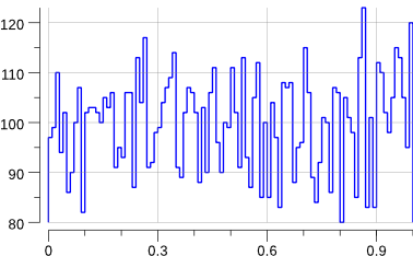
Indeed, that looks rather flat.

So far, so good. Let’s add a new distribution: the standard normal distribution.

func main() {
	const seed = 12345
	src := rand.NewSource(seed)
	rnd := rand.New(src)

	const N = 10000

	huni := hbook.NewH1D(100, 0, 1.0)
	hgauss := hbook.NewH1D(100, -5, 5)

	for i := 0; i < N; i++ {
		r := rnd.Float64() // r is in [0.0, 1.0)
		huni.Fill(r, 1)

		g := rnd.NormFloat64()
		hgauss.Fill(g, 1)
	}

	plot(huni, "uniform.png")
	plot(hgauss, "norm.png")
}

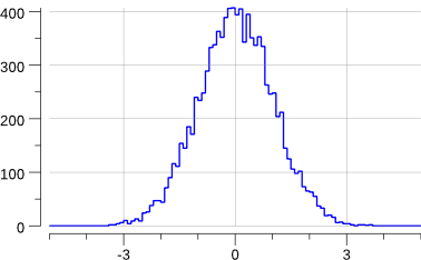
Running the code creates the following new plot:

$> go run ./mc-2.go

plot-norm

Note that this has slightly changed the previous "uniform.png" plot: we are sharing the source of random numbers between the 2 histograms. The sequence of random numbers is exactly the same than before (modulo the fact that now we generate -at least- twice the number than previously) but they are not associated to the same histograms.

OK, this does generate a gaussian. But what if we want to generate a gaussian with a mean other than 0 and/or a standard deviation other than 1 ?

The math/rand.NormFloat64 documentation kindly tells us how to achieve this:

“To produce a different normal distribution, callers can adjust the output using: sample = NormFloat64() * desiredStdDev + desiredMean

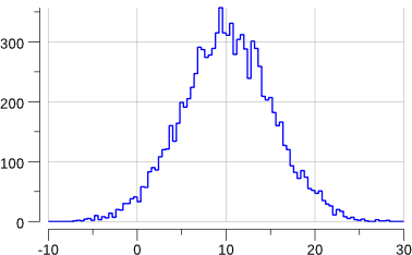
Let’s try to generate a gaussian of mean 10 and standard deviation 2. We’ll have to change a bit the definition of our histogram:

func main() {
	const seed = 12345
	src := rand.NewSource(seed)
	rnd := rand.New(src)

	const (
		N      = 10000
		mean   = 10.0
		stddev = 5.0
	)

	huni := hbook.NewH1D(100, 0, 1.0)
	hgauss := hbook.NewH1D(100, -10, 30)

	for i := 0; i < N; i++ {
		r := rnd.Float64() // r is in [0.0, 1.0)
		huni.Fill(r, 1)

		g := mean + stddev*rnd.NormFloat64()
		hgauss.Fill(g, 1)
	}

	plot(huni, "uniform.png")
	plot(hgauss, "gauss.png")

	fmt.Printf("gauss: mean=    %v\n", hgauss.XMean())
	fmt.Printf("gauss: std-dev= %v +/- %v\n", hgauss.XStdDev(), hgauss.XStdErr())
}

Running the program gives:

$> go run mc-3.go
gauss: mean=    10.105225624460644
gauss: std-dev= 5.048629091912316 +/- 0.05048629091912316

plot-gauss

OK enough for today. Next time, we’ll play a bit with math.Pi and Monte Carlo.

Note: all the code is go get-able via:

$> go get github.com/sbinet/blog/static/code/2017-10-11/...

10 Oct 2017, 11:07

L3 LEP data

Still working our way through this tutorial based on C++ and MINUIT:

http://www.desy.de/~rosem/flc_statistics/data/04_parameters_estimation-C.pdf

Now, we tackle the L3 LEP data. L3 was an experiment at the Large Electron Positron collider, at CERN, near Geneva. Until 2000, it recorded the decay products of e+e- collisions at center of mass energies up to 208 GeV.

An example is the muon pair production:

$$ e^+ e^- \rightarrow \mu^+\mu^-$$

Both muons are mainly detected and reconstructed from the tracking system. From the measurements, the curvature, charge and momentum are determined.

The file L3.dat contains recorded muon pair events. Every line is an event, a recorded collision of a \(e^+e^-\) pair producing a \(\mu^+\mu^-\) pair.

The first three columns contain the momentum components \(p_x\), \(p_y\) and \(p_z\) of the \(\mu^+\). The other three columns contain the momentum components for the \(mu^-\). Units are in \(GeV/c\).

Forward-Backward Asymmetry

An important parameter that constrains the Standard Model (the theoretical framework that models our current understanding of Physics) is the forward-backward asymmetry A:

$$ A = (N_F - N_B) / (N_F + N_B) $$

where:

  • \(N_F\) are the events in which the \(\mu^-\) flies forwards (\(\cos \theta_{\mu^-} > 0\));
  • \(N_B\) are the events in which the \(\mu^-\) flies backwards.

Given the L3.dat dataset, we would like to estimate the value of \(A\) and determine its statistical error.

In a simple counting experiment, we can write the statistical error as:

$$ \sigma_A = \sqrt{ \frac{(1-A^2)}{N} }$$

where \(N = N_F + N_B\).

So, as a first step, we can simply count the forward events.

First estimation

Let’s look at that data:

$> head -n 5 L3.dat
     4.584    -9.763   -18.508   -24.171    50.464    95.865
    62.570   184.448  -175.983   -28.392   -83.491    70.656
     7.387   101.650    13.531    -7.853  -108.002   -14.472
    43.672    56.083   -77.367   -40.893   -52.481    72.804
   -36.620   -60.832   -46.156    35.863    59.591    -3.220

First we need to assemble a bit of code to read in that file:

func read(fname string) []float64 {
	f, err := os.Open(fname)
	if err != nil {
		log.Fatal(err)
	}
	defer f.Close()

	var costh []float64
	sc := bufio.NewScanner(f)
	for sc.Scan() {
		var pp, pm [3]float64
		_, err = fmt.Sscanf(
			sc.Text(), "%f %f %f %f %f %f",
			&pp[0], &pp[1], &pp[2],
			&pm[0], &pm[1], &pm[2],
		)
		if err != nil {
			log.Fatal(err)
		}
		v := pm[0]*pm[0] + pm[1]*pm[1] + pm[2]*pm[2]
		costh = append(
			costh,
			pm[2]/math.Sqrt(v),
		)
	}

	if err := sc.Err(); err != nil {
		log.Fatal(err)
	}

	plot(costh)
	return costh
}

Now, with the \(\cos \theta_{\mu^{-}}\) calculation out of the way, we can actually compute the asymmetry and its associated statistical error:

func asym(costh []float64) (float64, float64) {
	n := float64(len(costh))
	nf := 0
	for _, v := range costh {
		if v > 0 {
			nf++
		}
	}

	a := 2*float64(nf)/n - 1
	sig := math.Sqrt((1 - a*a) / n)
	return a, sig
}

Running the code gives:

events: 346
A = 0.231 +/- 0.052

plot

OK. Let’s try to use gonum/optimize and a log-likelihood.

Estimation with gonum/optimize

To let optimize.Minimize loose on our dataset, we need the angular distribution:

$$ f(\theta, A) = \frac{3}{8} (1 + \cos^2 \theta) + A \cos\theta $$

we just need to feed that through the log-likelihood procedure:

func main() {
	costh := read("L3.dat")
	log.Printf("events: %d\n", len(costh))
	a, sig := asym(costh)
	log.Printf("A= %5.3f +/- %5.3f\n", a, sig)

	fcn := func(x []float64) float64 {
		lnL := 0.0
		A := x[0]
		const k = 3.0 / 8.0
		for _, v := range costh {
			lnL += math.Log(k*(1+v*v) + A*v)
		}
		return -lnL
	}

	grad := func(grad, x []float64) {
		fd.Gradient(grad, fcn, x, nil)
	}

	hess := func(h mat.MutableSymmetric, x []float64) {
		fd.Hessian(h.(*mat.SymDense), fcn, x, nil)
	}

	p := optimize.Problem{
		Func: fcn,
		Grad: grad,
		Hess: hess,
	}

	var meth = &optimize.Newton{}
	var p0 = []float64{0} // initial value for A

	res, err := optimize.Minimize(p, p0, nil, meth)
	if err != nil {
		log.Fatal(err)
	}
	display(res, p)
}

which, when run, gives:

$> go build -o fba fba.go
$> ./fba
events: 346
A= 0.231 +/- 0.052

results: &optimize.Result{Location:optimize.Location{X:[]float64{0.21964440563754575}, F:230.8167059887097, Gradient:[]float64{0}, Hessian:(*mat.SymDense)(0xc42004b440)}, Stats:optimize.Stats{MajorIterations:4, FuncEvaluations:5, GradEvaluations:5, HessEvaluations:5, Runtime:584120}, Status:4}

minimal function value:  230.817
number of parameters: 1
grad=[0]
hess=[429.2102851867676]
errs= [0.04826862636461834]
par-000: 2.196444e-01 +/- 4.826863e-02

ie: the same answer than the MINUIT-based code there:

Results of MINUIT minimisation
-------------------------------------

 Minimal function value:               230.817  
 Estimated difference to true minimum:   9.044e-11 
 Number of parameters:           1     
 Error definition (Fmin + Delta):         0.500  
 Exact covariance matrix.

   Parameter     Value       Error    positive    negative    L_BND    U_BND
 0          A  2.196e-01  4.827e-02 +4.767e-02 -4.879e-02  0.0e+00  0.0e+00

Covariance matrix: 
  2.330e-03

Correlation matrix: 
  1.000

09 Oct 2017, 11:11

Introduction to Minimization with Gonum

Switching gears a bit with regard to last week, let’s investigate how to perform minimization with Gonum.

In High Energy Physics, there is a program to calculate numerically:

  • a function minimum of \(F(a)\) of parameters \(a_i\) (with up to 50 parameters),
  • the covariance matrix of these parameters
  • the (asymmetric or parabolic) errors of the parameters from \(F_{min}+\Delta\) for arbitrary \(\Delta\)
  • the contours of parameter pairs \(a_i, a_j\).

This program is called MINUIT and was originally written by Fred JAMES in FORTRAN. MINUIT has been since then rewritten in C++ and is available through ROOT.

Let’s see what Gonum and its gonum/optimize package have to offer.

Physics example

Let’s consider a radioactive source. n measurements are taken, under the same conditions. The physicist measured and counted the number of decays in a given constant time interval:

rs := []float64{1, 1, 5, 4, 2, 0, 3, 2, 4, 1, 2, 1, 1, 0, 1, 1, 2, 1}

What is the mean number of decays ?

A naive approach could be to just use the (weighted) arithmetic mean:

mean := stat.Mean(rs, nil)
merr := math.Sqrt(mean / float64(len(rs)))
fmt.Printf("mean=  %v\n", mean)
fmt.Printf("µ-err= %v\n", merr)
// Output:
// mean=  1.7777777777777777
// µ-err= 0.31426968052735443 

Let’s plot the data:

func plot(rs []float64) {
	mean := stat.Mean(rs, nil)

	// hbook is go-hep.org/x/hep/hbook.
	// here we create a 1-dim histogram with 10 bins,
	// from 0 to 10.
	h := hbook.NewH1D(10, 0, 10)
	for _, x := range rs {
		h.Fill(x, 1)
	}
	h.Scale(1 / h.Integral())

	// hplot is a convenience package built on top
	// of gonum.org/v1/plot.
	// hplot is go-hep.org/x/hep/hplot.
	p := hplot.New()
	p.X.Label.Text = "r"
	hh := hplot.NewH1D(h)
	hh.FillColor = color.RGBA{255, 0, 0, 255}
	p.Add(hh)

	fct := hplot.NewFunction(distuv.Poisson{Lambda: mean}.Prob)
	fct.Color = color.RGBA{0, 0, 255, 255}
	p.Add(fct)
	p.Add(hplot.NewGrid())

	err := p.Save(10*vg.Centimeter, -1, "plot.png")
	if err != nil {
		log.Fatal(err)
	}
}

which gives:

plot

Ok, let’s try to estimate µ using a log-likelihood minimization.

With MINUIT

From the plot above and from first principles, we can assume a Poisson distribution. The Poisson probability is:

$$P(n|\mu) = \frac{\mu^{n}}{n!} e^{-\mu}$$

This therefore leads to a log-likelihood of:

$$\ln L(\mu) = n \ln(\mu) - \ln(n!) - \mu$$

which is the quantity we’ll try to optimize.

In C++, this would look like:

#include <math.h>
#include <cstdio>
#include "TMinuit.h"

#define NDATA 18
int r[NDATA]    = {1,1,  5, 4,2,0,3,2, 4,1,2,1,1,0,1,1,2,1};
int rfac[NDATA] = {1,1,120,24,2,1,6,2,24,1,2,1,1,1,1,1,2,1};

void fcn(int &npar, double *gin, double &f, double *par, int iflag) {
	int i;
	double mu, lnL;

	mu = par[0];
	lnL = 0.0;
	for (i=0; i<NDATA; i++) {
		lnL += r[i]*std::log(mu) - mu - std::log((double)rfac[i]);
	}
	f = -lnL;
}

int main(int argc, char **argv) {

	double arglist[10];
	int ierflg = 0;

	double start = 1.0; // initial value for mu
	double step = 0.1;
	double l_bnd = 0.1;
	double u_bnd = 10.;

	TMinuit minuit(1); // 1==number of parameters
	minuit.SetFCN(fcn);
	minuit.mnparm(
		0, "Poisson mu",
		start, step,
		l_bnd, u_bnd, ierflg
	);

	// set a 1-sigma error for the log-likelihood
	arglist[0] = 0.5;
	minuit.mnexcm("SET ERR",arglist,1,ierflg);

	// search for minimum.
	// computes covariance matrix and computes parabolic
	// errors for all parameters.
	minuit.mnexcm("MIGRAD",arglist,0,ierflg);

	// calculates exact, asymmetric errors for all
	// variable parameters.
	minuit.mnexcm("MINOS",arglist,0,ierflg);

	// set a 2-sigma error for the log-likelihood
	arglist[0] = 2.0;
	minuit.mnexcm("SET ERR",arglist,1,ierflg);

	// calculates exact, asymmetric errors for all
	// variable parameters.
	minuit.mnexcm("MINOS",arglist,0,ierflg);

	results(&minuit);
	return 0;
}

As this isn’t a blog post about how to use MINUIT, we won’t go too much into details.

Compiling the above program with:

$> c++ -o radio `root-config --libs --cflags` -lMinuit radio.cc

and then running it, gives:

$> ./radio
[...]
Results of MINUIT minimisation
-------------------------------------

 Minimal function value:                29.296  
 Estimated difference to true minimum:   2.590e-09 
 Number of parameters:           1     
 Error definition (Fmin + Delta):         2.000  
 Exact covariance matrix.

   Parameter     Value       Error    positive    negative    L_BND    U_BND
 0 Poisson mu  1.778e+00  6.285e-01 +7.047e-01 -5.567e-01  1.0e-01  1.0e+01

Covariance matrix: 
  3.951e-01

Correlation matrix: 
  1.000

So the mean of the Poisson distribution is estimated to 1.778 +/- 0.629.

With gonum/optimize

func main() {
	rs := []float64{1, 1, 5, 4, 2, 0, 3, 2, 4, 1, 2, 1, 1, 0, 1, 1, 2, 1}
	rfac := []float64{1, 1, 120, 24, 2, 1, 6, 2, 24, 1, 2, 1, 1, 1, 1, 1, 2, 1}

	mean := stat.Mean(rs, nil)
	merr := math.Sqrt(mean / float64(len(rs)))

	fmt.Printf("mean=%v\n", mean)
	fmt.Printf("merr=%v\n", merr)

	fcn := func(x []float64) float64 {
		mu := x[0]
		lnl := 0.0
		for i := range rs {
			lnl += rs[i]*math.Log(mu) - mu - math.Log(rfac[i])
		}
		return -lnl
	}

	grad := func(grad, x []float64) {
		fd.Gradient(grad, fcn, x, nil)
	}

	hess := func(h mat.MutableSymmetric, x []float64) {
		fd.Hessian(h.(*mat.SymDense), fcn, x, nil)
	}

	p := optimize.Problem{
		Func: fcn,
		Grad: grad,
		Hess: hess,
	}

	var meth = &optimize.Newton{}
	var p0 = []float64{1} // initial value for mu

	res, err := optimize.Minimize(p, p0, nil, meth)
	if err != nil {
		log.Fatal(err)
	}

	display(res, p)
	plot(rs)
}

Compiling and running this program gives:

$> go build -o radio radio.go
$> ./radio
mean=1.7777777777777777
merr=0.31426968052735443

results: &optimize.Result{Location:optimize.Location{X:[]float64{1.7777777839915905}, F:29.296294958031794, Gradient:[]float64{1.7763568394002505e-07}, Hessian:(*mat.SymDense)(0xc42022a000)}, Stats:optimize.Stats{MajorIterations:6, FuncEvaluations:9, GradEvaluations:7, HessEvaluations:7, Runtime:191657}, Status:4}

minimal function value:   29.296
number of parameters: 1
grad=[1.7763568394002505e-07]
hess=[10.123388051986694]
errs= [0.3142947001265352]

par-000: 1.777778e+00 +/- 6.285894e-01

Same result. Yeah!

gonum/optimize doesn’t try to automatically numerically compute the first- and second-derivative of an objective function (MINUIT does.) But using gonum/diff/fd, it’s rather easy to provide it to gonum/optimize.

gonum/optimize.Result only exposes the following informations (through gonum/optimize.Location):

// Location represents a location in the optimization procedure.
type Location struct {
	X        []float64
	F        float64
	Gradient []float64
	Hessian  *mat.SymDense
}

where X is the parameter(s) estimation and F the value of the objective function at X.

So we have to do some additional work to extract the error estimations on the parameters. This is done by inverting the Hessian to get the covariance matrix. The error on the i-th parameter is then:

erri := math.Sqrt(errmat.At(i,i)).

And voila.

Exercize for the reader: build a MINUIT-like interface on top of gonum/optimize that provides all the error analysis for free.

Next time, we’ll analyse a LEP data sample and use gonum/optimize to estimate a physics quantity.

NB: the material and orignal data for this blog post has been extracted from: http://www.desy.de/~rosem/flc_statistics/data/04_parameters_estimation-C.pdf.

04 Oct 2017, 11:17

Introduction to Statistics With Gonum

Starting a bit of a new series (hopefully with more posts than with the interpreter ones) about using Gonum to apply statistics.

This first post is really just a copy-paste of this one:

https://mubaris.com/2017-09-09/introduction-to-statistics-using-numpy

but using Go and Gonum instead of Python and numpy.

Go & Gonum

Gonum is “a set of packages designed to make writing numeric and scientific algorithms productive, performant and scalable.”

Before being able to use Gonum, we need to install Go. We can download and install the Go toolchain for a variety of platforms and operating systems from golang.org/dl.

Once that has been done, installing Gonum and all its dependencies can be done with:

$> go get gonum.org/v1/gonum/...

If you had a previous installation of Gonum, you can re-install it and update it to the latest one like so:

$> go get -u gonum.org/v1/gonum/...

Gonum and statistics

Gonum provides many statistical functions. Let’s use it to calculate the mean, median, standard deviation and variance of a small dataset.

// file: stats.go

package main

import (
	"fmt"
	"math"
	"sort"

	"gonum.org/v1/gonum/stat"
)

func main() {
	xs := []float64{
		32.32, 56.98, 21.52, 44.32,
		55.63, 13.75, 43.47, 43.34,
		12.34,
	}

	fmt.Printf("data: %v\n", xs)

	sort.Float64s(xs)
	fmt.Printf("data: %v (sorted)\n", xs)

	// computes the weighted mean of the dataset.
	// we don't have any weights (ie: all weights are 1)
	// so we just pass a nil slice.
	mean := stat.Mean(xs, nil)

	// computes the median of the dataset.
	// here as well, we pass a nil slice as weights.
	median := stat.Quantile(0.5, stat.Empirical, xs, nil)

	variance := stat.Variance(xs, nil)
	stddev := math.Sqrt(variance)

	fmt.Printf("mean=     %v\n", mean)
	fmt.Printf("median=   %v\n", median)
	fmt.Printf("variance= %v\n", variance)
	fmt.Printf("std-dev=  %v\n", stddev)
}

The program above performs some rather basic statistical operations on our dataset:

$> go run stats.go
data: [32.32 56.98 21.52 44.32 55.63 13.75 43.47 43.34 12.34]
data: [12.34 13.75 21.52 32.32 43.34 43.47 44.32 55.63 56.98] (sorted)
mean=     35.96333333333334
median=   43.34
variance= 285.306875
std-dev=  16.891029423927957

The astute reader will no doubt notice that the variance value displayed here differs from the one obtained with numpy.var:

>>> xs=[32.32, 56.98, 21.52, 44.32, 55.63, 13.75, 43.47, 43.34, 12.34]
>>> xs.sort()
>>> np.mean(xs)
35.963333333333338
>>> np.median(xs)
43.340000000000003
>>> np.var(xs)
253.60611111111109
>>> np.std(xs)
15.925015262507948

This is because numpy.var uses len(xs) as the divisor while gonum/stats uses the unbiased sample variance (ie: the divisor is len(xs)-1):

>>> np.var(xs, ddof=1)
285.30687499999999
>>> np.std(x, ddof=1)
16.891029423927957

With this quite blunt tool, we can analyse some real data from real life. We will use a dataset pertaining to the salary of European developers, all 1147 of them :). We have this dataset in a file named salary.txt.

// file: stats-salary.go

package main

import (
	"bufio"
	"fmt"
	"log"
	"math"
	"os"
	"sort"

	"gonum.org/v1/gonum/stat"
)

func main() {
	f, err := os.Open("salary.txt")
	if err != nil {
		log.Fatal(err)
	}
	defer f.Close()

	var xs []float64
	scan := bufio.NewScanner(f)
	for scan.Scan() {
		var v float64
		txt := scan.Text()
		_, err = fmt.Sscanf(txt, "%f", &v)
		if err != nil {
			log.Fatalf(
				"could not convert to float64 %q: %v",
				txt, err,
			)
		}
		xs = append(xs, v)
	}

	// make sure scanning the file and extracting values
	// went fine, without any error.
	if err = scan.Err(); err != nil {
		log.Fatalf("error scanning file: %v", err)
	}

	fmt.Printf("data sample size: %v\n", len(xs))

	sort.Float64s(xs)

	mean := stat.Mean(xs, nil)
	median := stat.Quantile(0.5, stat.Empirical, xs, nil)
	variance := stat.Variance(xs, nil)
	stddev := math.Sqrt(variance)

	fmt.Printf("mean=     %v\n", mean)
	fmt.Printf("median=   %v\n", median)
	fmt.Printf("variance= %v\n", variance)
	fmt.Printf("std-dev=  %v\n", stddev)
}

And here is the output:

$> go run ./stats-salary.go
data sample size: 1147
mean=     55894.53879686138
median=   48000
variance= 3.0464263289031615e+09
std-dev=  55194.44110508921

The data file can be obtained from here: salary.txt together with a much more detailed one there: salary.csv.