Switching gears a bit with regard to last week, let’s investigate how to perform minimization with Gonum.
In High Energy Physics, there is a program to calculate numerically:
- a function minimum of
\(F(a)\)of parameters\(a_i\)(with up to 50 parameters), - the covariance matrix of these parameters
- the (asymmetric or parabolic) errors of the parameters from
\(F_{min}+\Delta\)for arbitrary\(\Delta\) - the contours of parameter pairs
\(a_i, a_j\).
This program is called MINUIT and was originally written by Fred JAMES in FORTRAN.
MINUIT has been since then rewritten in C++ and is available through ROOT.
Let’s see what Gonum and its gonum/optimize package have to offer.
Physics example
Let’s consider a radioactive source.
n measurements are taken, under the same conditions.
The physicist measured and counted the number of decays in a given constant time interval:
rs := []float64{1, 1, 5, 4, 2, 0, 3, 2, 4, 1, 2, 1, 1, 0, 1, 1, 2, 1}
What is the mean number of decays ?
A naive approach could be to just use the (weighted) arithmetic mean:
mean := stat.Mean(rs, nil)
merr := math.Sqrt(mean / float64(len(rs)))
fmt.Printf("mean=  %v\n", mean)
fmt.Printf("µ-err= %v\n", merr)
// Output:
// mean=  1.7777777777777777
// µ-err= 0.31426968052735443
Let’s plot the data:
func plot(rs []float64) {
	mean := stat.Mean(rs, nil)

	// hbook is go-hep.org/x/hep/hbook.
	// here we create a 1-dim histogram with 10 bins,
	// from 0 to 10.
	h := hbook.NewH1D(10, 0, 10)
	for _, x := range rs {
		h.Fill(x, 1)
	}
	h.Scale(1 / h.Integral())

	// hplot is a convenience package built on top
	// of gonum.org/v1/plot.
	// hplot is go-hep.org/x/hep/hplot.
	p := hplot.New()
	p.X.Label.Text = "r"
	hh := hplot.NewH1D(h)
	hh.FillColor = color.RGBA{255, 0, 0, 255}
	p.Add(hh)

	fct := hplot.NewFunction(distuv.Poisson{Lambda: mean}.Prob)
	fct.Color = color.RGBA{0, 0, 255, 255}
	p.Add(fct)
	p.Add(hplot.NewGrid())

	err := p.Save(10*vg.Centimeter, -1, "plot.png")
	if err != nil {
		log.Fatal(err)
	}
}
which gives:
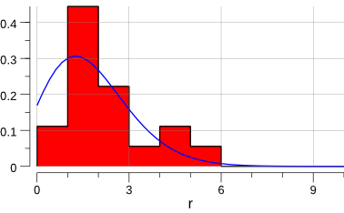
Ok, let’s try to estimate µ using a log-likelihood minimization.
With MINUIT
From the plot above and from first principles, we can assume a Poisson distribution. The Poisson probability is:
This therefore leads to a log-likelihood of:
which is the quantity we’ll try to optimize.
In C++, this would look like:
#include <math.h>
#include <cstdio>
#include "TMinuit.h"

#define NDATA 18
int r[NDATA]    = {1,1,  5, 4,2,0,3,2, 4,1,2,1,1,0,1,1,2,1};
int rfac[NDATA] = {1,1,120,24,2,1,6,2,24,1,2,1,1,1,1,1,2,1};

void fcn(int &npar, double *gin, double &f, double *par, int iflag) {
	int i;
	double mu, lnL;

	mu = par[0];
	lnL = 0.0;
	for (i=0; i<NDATA; i++) {
		lnL += r[i]*std::log(mu) - mu - std::log((double)rfac[i]);
	}
	f = -lnL;
}

int main(int argc, char **argv) {

	double arglist[10];
	int ierflg = 0;

	double start = 1.0; // initial value for mu
	double step = 0.1;
	double l_bnd = 0.1;
	double u_bnd = 10.;

	TMinuit minuit(1); // 1==number of parameters
	minuit.SetFCN(fcn);
	minuit.mnparm(
		0, "Poisson mu",
		start, step,
		l_bnd, u_bnd, ierflg
	);

	// set a 1-sigma error for the log-likelihood
	arglist[0] = 0.5;
	minuit.mnexcm("SET ERR",arglist,1,ierflg);

	// search for minimum.
	// computes covariance matrix and computes parabolic
	// errors for all parameters.
	minuit.mnexcm("MIGRAD",arglist,0,ierflg);

	// calculates exact, asymmetric errors for all
	// variable parameters.
	minuit.mnexcm("MINOS",arglist,0,ierflg);

	// set a 2-sigma error for the log-likelihood
	arglist[0] = 2.0;
	minuit.mnexcm("SET ERR",arglist,1,ierflg);

	// calculates exact, asymmetric errors for all
	// variable parameters.
	minuit.mnexcm("MINOS",arglist,0,ierflg);

	results(&minuit);
	return 0;
}
As this isn’t a blog post about how to use MINUIT, we won’t go too much into details.
Compiling the above program with:
$> c++ -o radio `root-config --libs --cflags` -lMinuit radio.cc
and then running it, gives:
$> ./radio
[...]
Results of MINUIT minimisation
-------------------------------------

 Minimal function value:                29.296
 Estimated difference to true minimum:   2.590e-09
 Number of parameters:           1
 Error definition (Fmin + Delta):         2.000
 Exact covariance matrix.

   Parameter     Value       Error    positive    negative    L_BND    U_BND
 0 Poisson mu  1.778e+00  6.285e-01 +7.047e-01 -5.567e-01  1.0e-01  1.0e+01

Covariance matrix:
  3.951e-01

Correlation matrix:
  1.000
So the mean of the Poisson distribution is estimated to 1.778 +/- 0.629.
With gonum/optimize
func main() {
	rs := []float64{1, 1, 5, 4, 2, 0, 3, 2, 4, 1, 2, 1, 1, 0, 1, 1, 2, 1}
	rfac := []float64{1, 1, 120, 24, 2, 1, 6, 2, 24, 1, 2, 1, 1, 1, 1, 1, 2, 1}

	mean := stat.Mean(rs, nil)
	merr := math.Sqrt(mean / float64(len(rs)))

	fmt.Printf("mean=%v\n", mean)
	fmt.Printf("merr=%v\n", merr)

	fcn := func(x []float64) float64 {
		mu := x[0]
		lnl := 0.0
		for i := range rs {
			lnl += rs[i]*math.Log(mu) - mu - math.Log(rfac[i])
		}
		return -lnl
	}

	grad := func(grad, x []float64) {
		fd.Gradient(grad, fcn, x, nil)
	}

	hess := func(h mat.MutableSymmetric, x []float64) {
		fd.Hessian(h.(*mat.SymDense), fcn, x, nil)
	}

	p := optimize.Problem{
		Func: fcn,
		Grad: grad,
		Hess: hess,
	}

	var meth = &optimize.Newton{}
	var p0 = []float64{1} // initial value for mu

	res, err := optimize.Minimize(p, p0, nil, meth)
	if err != nil {
		log.Fatal(err)
	}

	display(res, p)
	plot(rs)
}
Compiling and running this program gives:
$> go build -o radio radio.go
$> ./radio
mean=1.7777777777777777
merr=0.31426968052735443

results: &optimize.Result{Location:optimize.Location{X:[]float64{1.7777777839915905}, F:29.296294958031794, Gradient:[]float64{1.7763568394002505e-07}, Hessian:(*mat.SymDense)(0xc42022a000)}, Stats:optimize.Stats{MajorIterations:6, FuncEvaluations:9, GradEvaluations:7, HessEvaluations:7, Runtime:191657}, Status:4}

minimal function value:   29.296
number of parameters: 1
grad=[1.7763568394002505e-07]
hess=[10.123388051986694]
errs= [0.3142947001265352]

par-000: 1.777778e+00 +/- 6.285894e-01
Same result. Yeah!
gonum/optimize doesn’t try to automatically numerically compute the first- and second-derivative of an objective function (MINUIT does.)
But using gonum/diff/fd, it’s rather easy to provide it to gonum/optimize.
gonum/optimize.Result only exposes the following informations (through gonum/optimize.Location):
// Location represents a location in the optimization procedure.
type Location struct {
	X        []float64
	F        float64
	Gradient []float64
	Hessian  *mat.SymDense
}
where X is the parameter(s) estimation and F the value of the objective function at X.
So we have to do some additional work to extract the error estimations on the parameters.
This is done by inverting the Hessian to get the covariance matrix.
The error on the i-th parameter is then:
erri := math.Sqrt(errmat.At(i,i)).
And voila.
Exercize for the reader: build a MINUIT-like interface on top of gonum/optimize that provides all the error analysis for free.
Next time, we’ll analyse a LEP data sample and use gonum/optimize to estimate a physics quantity.
NB: the material and orignal data for this blog post has been extracted from: http://www.desy.de/~rosem/flc_statistics/data/04_parameters_estimation-C.pdf.